In the previous topic we have covered the distributional apporach(which have high dimension vector to represent words and also sparse in nature) but in this post we will cover the Distributed apporach(which have low dimension vecotr and are dense in nature) and how to create word embedding using pretrained model.

Distributed Representation

To overcome the issue of high-dimensional representation and sparse vector to represent word, Distributed Representation help in these issue and therefore they have gained a lot of momentum in the past six to seven days. Different distributed representation are

Word Embedding

Word Embeddings are the texts converted into numbers. Embeddings translate large sparse vectors into a lower-dimensional space that preserves semantic relationships. Word embeddings is a technique where individual words of a domain or language are represented as real-valued vectors in a lower dimensional space and placing vectors of semantically similar items close to each other. This way words that have similar meaning have similar distances in the vector space as shown below.

“king is to queen as man is to woman” encoded in the vector space as well as verb Tense and Country and their capitals are encoded in low dimensional space preserving the semantic relationships.

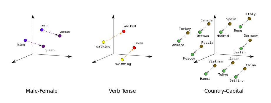
Word2vec is an algorithm invented at Google for training word embeddings. word2vec relies on the distributional hypothesis. The distributional hypothesis states that words which, often have the same neighboring words tend to be semantically similar. This helps to map semantically similar words to geometrically close embedding vectors.

Now the question arises that how we will create word embedding?

Well we can also use pre-trained word embedding arcitecture or we can also train our own word embedding.

Pre-trained word embeddings

What is pre-trained word embeddings?

Pretrained Word Embeddings are the embeddings learned in one task that are used for solving another similar task.

These embeddings are trained on large datasets, saved, and then used for solving other tasks. That’s why pretrained word embeddings are a form of Transfer Learning.

Why do we need Pretrained Word Embeddings?

Pretrained word embeddings capture the semantic and syntactic meaning of a word as they are trained on large datasets. They are capable of boosting the performance of a Natural Language Processing (NLP) model. These word embeddings come in handy during hackathons and of course, in real-world problems as well.

But why should we not learn our own embeddings?

Well, learning word embeddings from scratch is a challenging problem due to two primary reasons:
- Sparsity of training data
- Large number of trainable parameters

With pretrained embedding you just need to download the embeddings and use it to get the vectors for the word you want.Such embeddings can be thought of as a large collection of key-value pairs, where keys are the words in the vocabulary and values are their corresponding word vectors. Some of the most popular pre-trained embeddings are Word2vec by Google, GloVe by Stanford, and fasttext embeddings by Facebook, to name a few. Further, they’re available for various dimensions like d = 25, 50, 100, 200, 300, 600.

Here is the code where we will find the words that are semantically most similar to the word "beautiful".

#Downdloading Google News vectors embeddings.
!wget -P /tmp/input/ -c "https://s3.amazonaws.com/dl4j-distribution/GoogleNews-vectors-negative300.bin.gz"

--2021-02-01 08:38:46--  https://s3.amazonaws.com/dl4j-distribution/GoogleNews-vectors-negative300.bin.gz
Resolving s3.amazonaws.com (s3.amazonaws.com)... 52.216.200.157
Connecting to s3.amazonaws.com (s3.amazonaws.com)|52.216.200.157|:443... connected.
HTTP request sent, awaiting response... 200 OK
Length: 1647046227 (1.5G) [application/x-gzip]
Saving to: ‘/tmp/input/GoogleNews-vectors-negative300.bin.gz’

GoogleNews-vectors- 100%[===================>]   1.53G  46.1MB/s    in 35s     

2021-02-01 08:39:21 (45.3 MB/s) - ‘/tmp/input/GoogleNews-vectors-negative300.bin.gz’ saved [1647046227/1647046227]

from gensim.models import Word2Vec, KeyedVectors
pretrainedpath = '/tmp/input/GoogleNews-vectors-negative300.bin.gz'

w2v_model = KeyedVectors.load_word2vec_format(pretrainedpath, binary=True) #load the model
print("done loading word2vec")

print("Numver of words in vocablulary: ",len(w2v_model.vocab)) #Number of words in the vocabulary.

done loading word2vec
Numver of words in vocablulary:  3000000

w2v_model.most_similar('beautiful')

[('gorgeous', 0.8353004455566406),
 ('lovely', 0.810693621635437),
 ('stunningly_beautiful', 0.7329413890838623),
 ('breathtakingly_beautiful', 0.7231341004371643),
 ('wonderful', 0.6854087114334106),
 ('fabulous', 0.6700063943862915),
 ('loveliest', 0.6612576246261597),
 ('prettiest', 0.6595001816749573),
 ('beatiful', 0.6593326330184937),
 ('magnificent', 0.6591402292251587)]

Note that if we search for a word that is not present in the Word2vec model (e.g., “practicalnlp”), we’ll see a “key not found” error. Hence, as a good coding practice, it’s always advised to first check if the word is present in the model’s vocabulary before attempting to retrieve its vector.

w2v_model['practicalnlp']

---------------------------------------------------------------------------
KeyError                                  Traceback (most recent call last)
<ipython-input-4-354849ef77a2> in <module>()
      1 #What if I am looking for a word that is not in this vocabulary?
----> 2 w2v_model['practicalnlp']

/usr/local/lib/python3.6/dist-packages/gensim/models/keyedvectors.py in __getitem__(self, entities)
    335         if isinstance(entities, string_types):
    336             # allow calls like trained_model['office'], as a shorthand for trained_model[['office']]
--> 337             return self.get_vector(entities)
    338 
    339         return vstack([self.get_vector(entity) for entity in entities])

/usr/local/lib/python3.6/dist-packages/gensim/models/keyedvectors.py in get_vector(self, word)
    453 
    454     def get_vector(self, word):
--> 455         return self.word_vec(word)
    456 
    457     def words_closer_than(self, w1, w2):

/usr/local/lib/python3.6/dist-packages/gensim/models/keyedvectors.py in word_vec(self, word, use_norm)
    450             return result
    451         else:
--> 452             raise KeyError("word '%s' not in vocabulary" % word)
    453 
    454     def get_vector(self, word):

KeyError: "word 'practicalnlp' not in vocabulary"

If you’re new to embeddings, always start by using pre-trained word embeddings in your project. Understand their pros and cons, then start thinking of building your own embeddings. Using pre-trained embeddings will quickly give you a strong baseline for the task at hand.

In the next blog post we will cover the Training our own emdeddings models.

TRAINING OUR OWN EMBEDDINGS

For training our own word embeddings we’ll look at two architectural variants that were propossed in Word2Vec

Continuous bag of words(CBOW)
SkipGram

Continuous Bag of Words

CBOW tries to learn a language model that tries to predict the “center” word from the words in its context. Let’s understand this using our toy corpus(the quick brown fox jumped over the lazy dog). If we take the word “jumps” as the center word, then its context is formed by words in its vicinity. If we take the context size of 2, then for our example, the context is given by brown, fox, over, the. CBOW uses the context words to predict the target word—jumped. CBOW tries to do this for every word in the corpus; i.e., it takes every word in the corpus as the target word and tries to predict the target word from its corresponding context words.

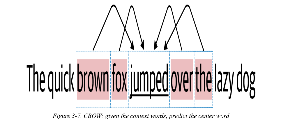
Understanding CBOW architecture

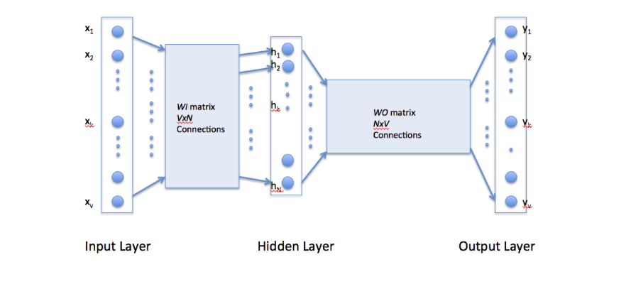
consider the training corpus having the following sentences:

“the dog saw a cat”, “the dog chased the cat”, “the cat climbed a tree”

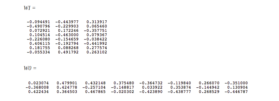
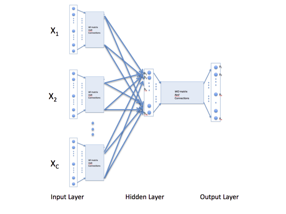
The corpus vocabulary has eight words. Once ordered alphabetically, each word can be referenced by its index. For this example, our neural network will have eight input neurons and eight output neurons. Let us assume that we decide to use three neurons in the hidden layer. This means that WI and WO will be 8×3 and 3×8 matrices, respectively. Before training begins, these matrices are initialized to small random values as is usual in neural network training. Just for the illustration sake, let us assume WI and WO to be initialized to the following values:

Suppose we want the network to learn relationship between the words “cat” and “climbed”. That is, the network should show a high probability for “climbed” when “cat” is inputted to the network. In word embedding terminology, the word “cat” is referred as the context word and the word “climbed” is referred as the target word. In this case, the input vector X will be [0 1 0 0 0 0 0 0]. Notice that only the second component of the vector is 1. This is because the input word is “cat” which is holding number two position in sorted list of corpus words. Given that the target word is “climbed”, the target vector will look like [0 0 0 1 0 0 0 0 ]t.

With the input vector representing “cat”, the output at the hidden layer neurons can be computed as

Ht = XtWI = [-0.490796 -0.229903 0.065460]

It should not surprise us that the vector H of hidden neuron outputs mimics the weights of the second row of WI matrix because of 1-out-of-V representation. So the function of the input to hidden layer connections is basically to copy the input word vector to hidden layer. Carrying out similar manipulations for hidden to output layer, the activation vector for output layer neurons can be written as

HtWO = [0.100934 -0.309331 -0.122361 -0.151399 0.143463 -0.051262 -0.079686 0.112928]

now we will use the formula

Thus, the probabilities for eight words in the corpus are:

[0.143073 0.094925 0.114441 0.111166 0.149289 0.122874 0.119431 0.144800]

The probability in bold is for the chosen target word “climbed”. Given the target vector is [0 0 0 1 0 0 0 0 ]

The above description and architecture is meant for learning relationships between pair of words. In the continuous bag of words model, context is represented by multiple words for a given target words. For example, we could use “cat” and “tree” as context words for “climbed” as the target word. This calls for a modification to the neural network architecture. The modification, shown below, consists of replicating the input to hidden layer connections C times, the number of context words, and adding a divide by C operation in the hidden layer neurons.

[An alert reader pointed that the figure below might lead some readers to think that CBOW learning uses several input matrices. It is not so. It is the same matrix, WI, that is receiving multiple input vectors representing different context words]

I can understand that things can be little hazy at first.But if you read this one more time it will be crystal clear.

In the next blog i will cover skip-gram and other text representation technique.

1. Notes are compiled from Practical Natural Language Processing: A Comprehensive Guide to Building Real-World NLP Systems, Medium,CBOW and Skip-gram and Code from github repo ↩

2. If you face any problem or have any feedback/suggestions feel free to comment.↩