Topic 03.1: Text Representation(PART-1)
Representing raw text to suitable numeric format
What is Text Representation?
In NLP the game is all about text. Text that we collect and provide to our computer.
But what if the text we provide cannot be comprehend by our NLP or machine Learning algorithm? Well this nightmare is true because as we know our algorithm cannot handle the text. It might not get the simple English(or any other language text) which we easily grasp.
Number is something that computer always love. So isn't it's better that we convert our text into suitable numeric format.
Conversion of raw text to a suitable numerical form is called text representation.
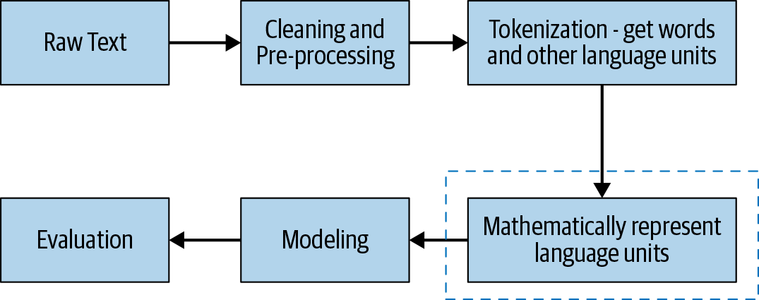
With respect to the larger picture for any NLP problem, the scope of this chapter is depicted by the dotted box in the below figure.

We will start with simple approaches and go all the way to state-of-the-art techniques for representing text. These approaches are classified into four categories:
- Basic vectorization approaches
- Distributed representations
- Universal language representation
- Handcrafted features
Before starting with Basic Vectorization approaches let me give you a clear picture about Vector space models.
Vector Space Model
- Text are represented with a vectors of numbers that are called Vector Space Model(VSM).
- VSM is fundamental to many information-retrieval operations, from scoring documents on a query to document classification and document clustering.
- It’s a mathematical model that represents text units as vectors.
- In the simplest form, these are vectors of identifiers, such as index numbers in a corpus vocabulary.
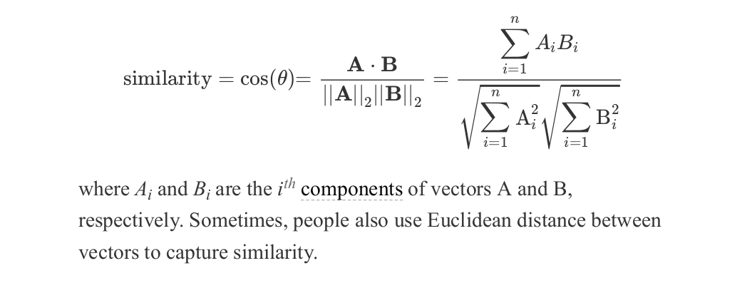
- In this setting, the most common way to calculate similarity between two text blobs is using cosine similarity.
Note: The cosine of the angle between their corresponding vectors. The cosine of 0° is 1 and the cosine of 180° is –1, with the cosine monotonically decreasing from 0° to 180°.Given two vectors, A and B, each with n components, the similarity between them is computed as follows:

Basic Vectorization Approaches
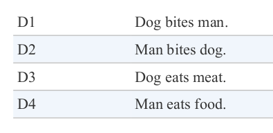
To understand different Basic vectorization approaches let’s take a toy corpus with only four documents—D 1 , D 2 , D 3 , D 4 —as an example.

The vocabulary of this corpus is comprised of six words: [dog, bites, man, eats, meat, food]. We can organize the vocabulary in any order. In this example, we simply take the order in which the words appear in the corpus.
1.One-Hot Encoding
- In one-hot encoding, each word w in the corpus vocabulary is given aunique integer ID w id that is between 1 and |V|, where V is the set of the corpus vocabulary.
- Each word is then represented by a V-dimensional binary vector of 0s and 1s. This is done via a |V| dimension vector filled with all 0s except the index, where index = w id .
- At this index, we simply put a 1. The representation for individual words is then combined to form a sentence representation.
Example of toy dataset:
- We first map each of the six words to unique IDs: dog = 1, bites = 2, man = 3, meat = 4 , food = 5, eats = 6.
- Now for D1 “dog bites man” each word is a six-dimensional vector.
- Dog is represented as [1 0 0 0 0 0], as the word “dog” is mapped to ID 1. Bites is represented as [0 1 0 0 0 0], and so on and so forth. Thus, D1 is represented as [ [1 0 0 0 0 0] [0 1 0 0 0 0] [0 0 1 0 0 0]].
- Other documents in the corpus can be represented similarly.
S1 = 'dog bites man'
S2 = 'man bites dog'
S3 = 'dog eats meat'
S4 = 'man eats food'
data = [S1.split(),S2.split(),S3.split(),S4.split()]
from sklearn.preprocessing import OneHotEncoder

#One-Hot Encoding
onehot_encoder = OneHotEncoder()
onehot_encoded = onehot_encoder.fit_transform(data).toarray()
print("Onehot Encoded Matrix:\n",onehot_encoded)
Pros of One-Hot Encoding
- one-hot encoding is intuitive to understand and straightforward to implement.
Cons of One-Hot Encoding
- The size of the vectors is directly proportional to the size of the vocabulary and also the vectors is sparse.
- There is no fixed length representation of text. Text with 10 words is much larger than text with 4 words.
- Semantic meaniing is poorly captured by One-Hot Ecnoding.
- Cannot handle out of vocabulary(OOV) problem.
Note: OOV is cause when we ecounter the words that are not present in the vocabulary.
2.Bag of Words
The key idea behind it is as follows:
- represent the text under consideration as a bag (collection) of words while ignoring the order and context.
- The basic intuition behind it is that it assumes that the text belonging to a given class in the dataset is characterized by a unique set of words.
- If two text pieces have nearly the same words, then they belong to the same bag (class). Thus, by analyzing the words present in a piece of text, one can identify the class (bag) it belongs to.
- BoW maps words to unique integer IDs between 1 and |V|.
- Each document in the corpus is then converted into a vector of |V| dimensions where in the i th component of the vector, i = w id , is simply the number of times the word w occurs in the document, i.e., we simply score each word in V by their occurrence count in the document.
Example of toy dataset:
- The word IDs are dog = 1, bites = 2, man = 3, meat = 4 , food = 5, eats = 6.
- So D1 becomes [1 1 1 0 0 0]. This is because the first three words in the vocabulary appeared exactly once in D1, and the last three did not appear at all.
- D4 becomes [0 0 1 0 1 1].
documents = ["Dog bites man.", "Man bites dog.", "Dog eats meat.", "Man eats food."] #Same as the earlier notebook
processed_docs = [doc.lower().replace(".","") for doc in documents]
processed_docs
from sklearn.feature_extraction.text import CountVectorizer

#look at the documents list
print("Our corpus: ", processed_docs)

count_vect = CountVectorizer()
#Build a BOW representation for the corpus
bow_rep = count_vect.fit_transform(processed_docs)

#Look at the vocabulary mapping
print("Our vocabulary: ", count_vect.vocabulary_)

#see the BOW rep for first 2 documents
print("BoW representation for 'dog bites man': ", bow_rep[0].toarray())
print("BoW representation for 'man bites dog: ",bow_rep[1].toarray())

#Get the representation using this vocabulary, for a new text
temp = count_vect.transform(["dog and dog are friends"])
print("Bow representation for 'dog and dog are friends':", temp.toarray())
~In the above code, we represented the text considering the frequency of words into account. However, sometimes, we don't care about frequency much, but only want to know whether a word appeared in a text or not. That is, each document is represented as a vector of 0s and 1s. We will use the option binary=True in CountVectorizer for this purpose.
count_vect = CountVectorizer(binary=True)
bow_rep_bin = count_vect.fit_transform(processed_docs)
temp = count_vect.transform(["dog and dog are friends"])
print("Bow representation for 'dog and dog are friends':", temp.toarray())
Pros of Bag of Words
- BoW is fairly simple to understand and implement.
- The text have similar length.
- documents having the same words will have their vector representations closer to each other as compared to documents with completely different words.BoW scheme captures the semantic similarity of documents. So if two documents have similar vocabulary, they’ll be closer to each other in the vector space and vice versa.
Cons of Bag of Words
- The size of the vectors is directly proportional to the size of the vocabulary and also the vectors is sparse.
- It does not capture the similarity between different words that mean the same thing. Say we have three documents: “I run”, “I ran”, and “I ate”. BoW vectors of all three documents will be equally apart.
- Cannot handle out of vocabulary(OOV) problem.
- In Bag of Words, words order are lost.
3.Bag of N-Grams
- The bag-of-n-grams (BoN) approach tries to remedy the notion of phrases or word ordering.
- This can help us capture some context, which earlier approaches could not do. Each chunk is called an n-gram.
- The corpus vocabulary, V, is then nothing but a collection of all unique n-grams across the text corpus.
- Then, each document in the corpus is represented by a vector of length |V|.
- This vector simply contains the frequency counts of n-grams present in the document and zero for the n-grams that are not present.
Example of toy dataset:
- Let’s construct a 2- gram (a.k.a. bigram) model for it.
- The set of all bigrams in the corpus is as follows: {dog bites, bites man, man bites, bites dog, dog eats, eats meat, man eats, eats food}.
- Then, BoN representation consists of an eight-dimensional vector for each document.
- The bigram representation for the first two documents is as follows: D 1 : [1,1,0,0,0,0,0,0], D 2 : [0,0,1,1,0,0,0,0].
- The other two documents follow similarly.
~CountVectorizer, which we used for BoW, can be used for getting a Bag of N-grams representation as well, using its ngram_range argument.
from sklearn.feature_extraction.text import CountVectorizer

#Ngram vectorization example with count vectorizer and uni, bi, trigrams
count_vect = CountVectorizer(ngram_range=(1,3))

#Build a BOW representation for the corpus
bow_rep = count_vect.fit_transform(processed_docs)

#Look at the vocabulary mapping
print("Our vocabulary: ", count_vect.vocabulary_)

#see the BOW rep for first 2 documents
print("BoW representation for 'dog bites man': ", bow_rep[0].toarray())
print("BoW representation for 'man bites dog: ",bow_rep[1].toarray())

#Get the representation using this vocabulary, for a new text
temp = count_vect.transform(["dog and dog are friends"])

print("Bow representation for 'dog and dog are friends':", temp.toarray())
Pros of Bag of N-Gram
- It captures some context and word-order information in the form of n-grams.
- Thus, resulting vector space is able to capture some semantic similarity.
Cons of Bag of N-Gram
- As n increases, dimensionality (and therefore sparsity) only increases rapidly.
- It still provides no way to address the OOV problem.
4.TF-IDF
TF-IDF, or term frequency–inverse document frequency assign importance to the word in the documents.
The intuition behind TF-IDF is as follows:
- if a word w appears many times in a document d i but does not occur much in the rest of the documents dj in the corpus, then the word w must be of great importance to the document di.
- The importance of w should increase in proportion to its frequency in di , but at the same time, its importance should decrease in proportion to the word’s frequency in other documents dj in the corpus.
- Mathematically, this is captured using two quantities: TF and IDF. The two are then combined to arrive at the TF-IDF score.
TF (term frequency)
- measures how often a term or word occurs in a given document.
- Since different documents in the corpus may be ofdifferent lengths, a term may occur more often in a longer document as compared to a shorter document.
- To normalize these counts, we divide the number of occurrences by the length of the document.
TF of a term t in a document d is defined as:

DF (inverse document frequency)
- measures the importance of the term across a corpus.
- In computing TF, all terms are given equal importance (weightage).
- However, it’s a well-known fact that stop words like is, are, am, etc., are not important, even though they occur frequently.
- To account for such cases, IDF weighs down the terms that are very common across a corpus and weighs up the rare terms.
IDF of a term t is calculated as follows:

Thus, TF-IDF score = TF * IDF.
from sklearn.feature_extraction.text import TfidfVectorizer

tfidf = TfidfVectorizer()
bow_rep_tfidf = tfidf.fit_transform(processed_docs)

#IDF for all words in the vocabulary
print("IDF for all words in the vocabulary",tfidf.idf_)
print("-"*10)
#All words in the vocabulary.
print("All words in the vocabulary",tfidf.get_feature_names())
print("-"*10)

#TFIDF representation for all documents in our corpus
print("TFIDF representation for all documents in our corpus\n",bow_rep_tfidf.toarray())
print("-"*10)

temp = tfidf.transform(["dog and man are friends"])
print("Tfidf representation for 'dog and man are friends':\n", temp.toarray())
Pros of TF-IDF
- Assign importance to the words in a particular documents.
Cons of TF-IDF
- The feature vectors are sparse and high-dimensional representations.
- They cannot handle OOV problem.
Well that now we have completed all the basic vectorization approach. In the next topic we will cover other approaches for text representation followed by state-of-art-approach.